Analysis of long-term performance

A.J. Erickson, P.T. Weiss, J.S. Gulliver, R.M. Hozalski

After assessment data from multiple storm events have been analyzed, the long-term performance of a stormwater treatment practice can be calculated. Long-term performance can be expressed as a single value for performance with associated uncertainty (e.g., average phosphorus capture = 72% ± 17% confidence interval for α = 0.05) or expressed graphically for the entire range of data (e.g., exceedance method). Applying both single-value and graphical approaches to monitoring data results is a detailed description of performance. Results from analysis of long-term performance represents only the period of time encompassed by the storm events (e.g., 3 months, 1 year, 2 years) and that specific treatment practice. Analysis of monitoring data from many storms can be used to investigate relationships between stormwater treatment practice performance and runoff intensity, pollutant load or concentration, or other variables.

Summation of load

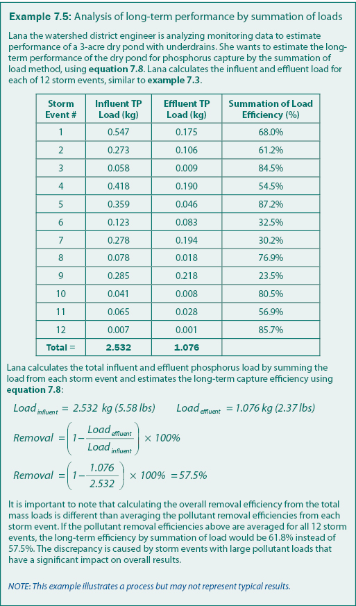
Analysis of long-term performance by summation of load is similar to analysis of a single storm event, except that the data are comprised of pollutant load from multiple storm events instead of loads from individual samples. To do this, influent and effluent load is calculated separately for each storm event using equation 7.7 as illustrated in example 7.3. Long-term performance can then be calculated using equation 7.8 with the total mass of influent load and total mass of effluent load being the sum of the influent and effluent mass load for all storm events.

In the summation of load method, the pollutant mass entering and exiting the stormwater treatment practice for each runoff event is summed, and the removal efficiency is computed from the total influent and effluent load. Thus, a storm with a relatively small pollutant load will contribute less to the total load than a storm with a relatively large pollutant load, as shown in example 7.5. Therefore, assessment data from a stormwater treatment practice that is analyzed using the summation of load method may be biased by storms with large pollutant load.

The average pollutant removal from the assessment of a given stormwater treatment practice’s long-term performance can be used to compare different time periods or watershed conditions: for the same stormwater treatment practice, to other stormwater treatment practices of the same type (e.g., dry pond vs. dry pond), or to other stormwater treatment practices (e.g., dry pond vs. rain garden). Removal efficiencies obtained from the assessment of long-term performance can also be compared with efficiencies obtained from other analysis methods (e.g., EMC efficiency), as described in the next section and shown in example 7.6.

Event mean concentration efficiency

Analysis of long-term performance by the event mean concentration (EMC) efficiency method involves calculating the influent and effluent EMC for each storm event (equation 7.13, example 7.4), determining the average influent and effluent EMC from all storms, and calculating the long-term performance as the percent reduction in concentration based on the average influent and effluent EMC (U.S. EPA 2002). Long-term removal efficiency by the EMC method can be calculated using equation 7.16 for all storm events, as shown in example 7.6.

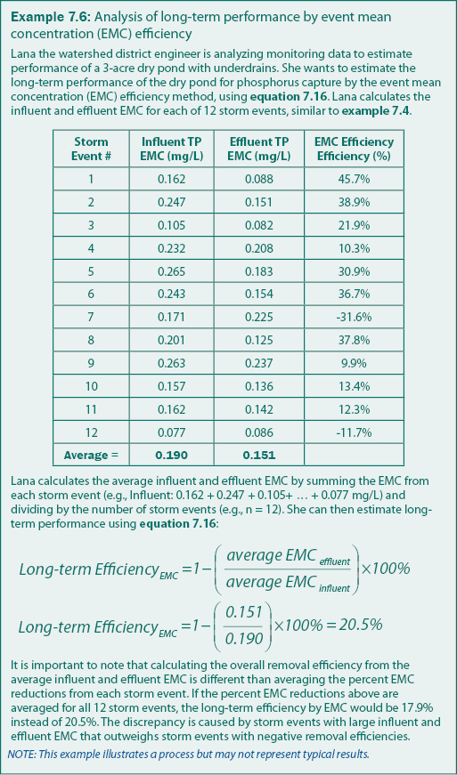
The stormwater treatment practice long-term efficiency results from examples 7.5 and 7.6 are significantly different. During the 12 storm events that were monitored, 57.5% of the pollutant load was removed by the stormwater treatment practice but the average EMC, however, is only reduced on average by 20.5%. As discussed in Analysis of Individual Storm Events, discrepancies between summation of load and EMC efficiency is caused by significant water budget components (e.g., infiltration, evapotranspiration) that are not necessarily accounted for by the analysis methods. For the data shown in examples 7.2, 7.3, and 7.4, it can be concluded that a water budget export component (e.g., infiltration) is significant but not accounted for due to the estimated 28.3% runoff volume reduction. Infiltration of stormwater within a treatment practice will reduce the mass of dissolved pollutants (e.g., due to adsorption in the soils) but is not likely to reduce the EMC in the effluent because both the volume of runoff and the dissolved pollutants are infiltrating. This conclusion is only possible because the data was analyzed using three methods; volume reduction, summation of load, and the EMC efficiency methods. Typically, the long-term performance as estimated by the summation of load method is numerically larger than the EMC efficiency (e.g., 57.5% vs. 20.5%). If there is no addition or loss of water (e.g., due to direct rainfall, evaporation, infiltration, etc.), then the summation of load and event mean concentration methods will yield identical performance estimations.

Estimating uncertainty

The uncertainty of long-term performance analysis by summation of load and event mean concentration (EMC) is related to the total number and variation of storms assessed, but it is independent of the method used to calculate performance. With all other variables held constant, the uncertainty in the average percent removal decreases as the number of analyzed storm events increases. One requirement for calculating uncertainty is that a percent removal and standard deviation for all incorporated storm events can be calculated.

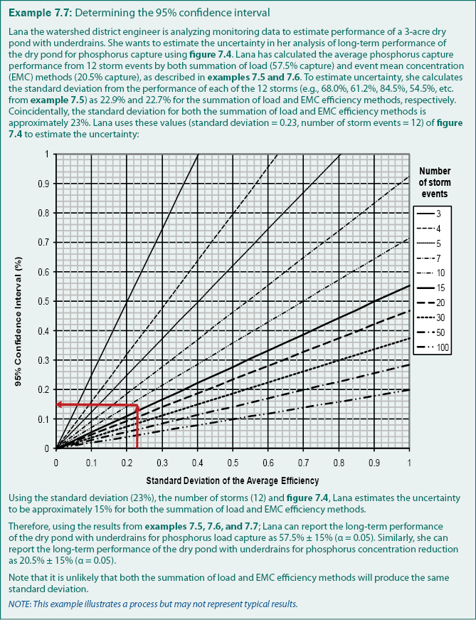
The 95% confidence interval is recommended to adequately represent uncertainty in average pollutant removal efficiency because it indicates that there is a 95% probability that the actual average performance will be within the confidence interval. For example, a stormwater treatment practice with an average pollutant capture rate of 72% ± 17% confidence interval (α = 0.05) will have a 95% (19 out of 20) probability that the actual average pollutant capture rate is between 55% and 89%. The range of the confidence interval (in this case, ± 17% for α = 0.05) is dependent on the standard deviation and the number of monitored storm events. The relationship between standard deviation, number of storm events, and 95% confidence interval is shown in figure 7.4.

A simple method (equation 7.17) for calculating uncertainty is based on the Student (Gosset) t-distribution. The Student t-distribution, given in table 7.1, is a probability distribution used to estimate the average of a normally-distributed population from a sample of the population and is more accurate than the similar z-distribution for small (n < 30) sample sizes. Thus, the Student t-distribution is used because the number of storms assessed will likely be fewer than 30. For more information on distributions, consult a statistics text (e.g., MacBerthouex and Brown 1996, Moore and McCabe 2003).

Uncertainty can be calculated by equation 7.17 using the number of storm events, the standard deviation of the performance data, and the Student t value (from Table 7.1). The standard deviation can be calculated in Microsoft Excel™ (stdev function) or as described in many statistical textbooks. The Student t value can also be obtained in Microsoft Excel™ (tinv function) or from table 7.1 using the degrees of freedom (d.f. = n-1) and the probability of failure (α). For the 95% confidence interval, α = 0.05. For example, if n = 15, the Student t value for the 67% confidence interval would be 1.00 (d.f. = 14, α = 0.33). Alternatively, uncertainty can be estimated directly using figure 7.4 for a known standard deviation, number of storm events, and an assumed 95% confidence interval, as shown in example 7.7.

Exceedance Method

The exceedance method is a graphical representation of long-term performance and is especially useful in calculating expected effluent characteristics (e.g., pollutant concentration, runoff volume) and visually comparing and illustrating trends in performance over the range of data values (e.g., runoff volume, flow rate, pollutant concentration, or pollutant load). This method does not, however, result in a single value of performance for easy comparison to other monitoring data (other sites, time periods, etc.) but can be graphically compared to other monitoring data. Monitoring data can be compared using the exceedance method by graphical comparison (e.g., plotting inflow and outflow for multiple practices) or by comparing performance a several exceedance levels (e.g., 10%, 50%, and 90% exceedance).

Pollutant removal can be estimated by integrating the curve or best-fit distribution function for both the inflow and outflow data, and then calculating the difference between in the inflow and outflow volumes, pollutant mass loads, pollutant concentrations, or other variables as listed below. Due to the complexity of this method, it is more common to report performance for several exceedances (i.e., inflow and outflow data for 10%, 50%, and 90% exceedance) or report the percent exceedance for specific outflow goals (e.g., target volume, concentration, or load).

The exceedance method is applied to monitoring data by first determining whether the difference between influent and effluent measurements is statistically significant and then plotting the data on a percent exceedance plot. Methods for applying the appropriate non-parametric (or parametric, if applicable) statistical tests can be found in many statistical texts and are not described here. Plotting the data on an exceedance plot in a spreadsheet program requires entering the data, ranking the inflow and outflow data separately in increasing order, calculating the percent exceedance for each data point (equation 7.18), and plotting the data on a normal or log-normal plot of parameter versus percent exceedance. In order to make defensible conclusions or predictions from the exceedance method, several data points (at least 5, more than 10 recommended) are necessary. An example of plotting and interpreting results from monitoring data using the exceedance method is shown in example 7.8.

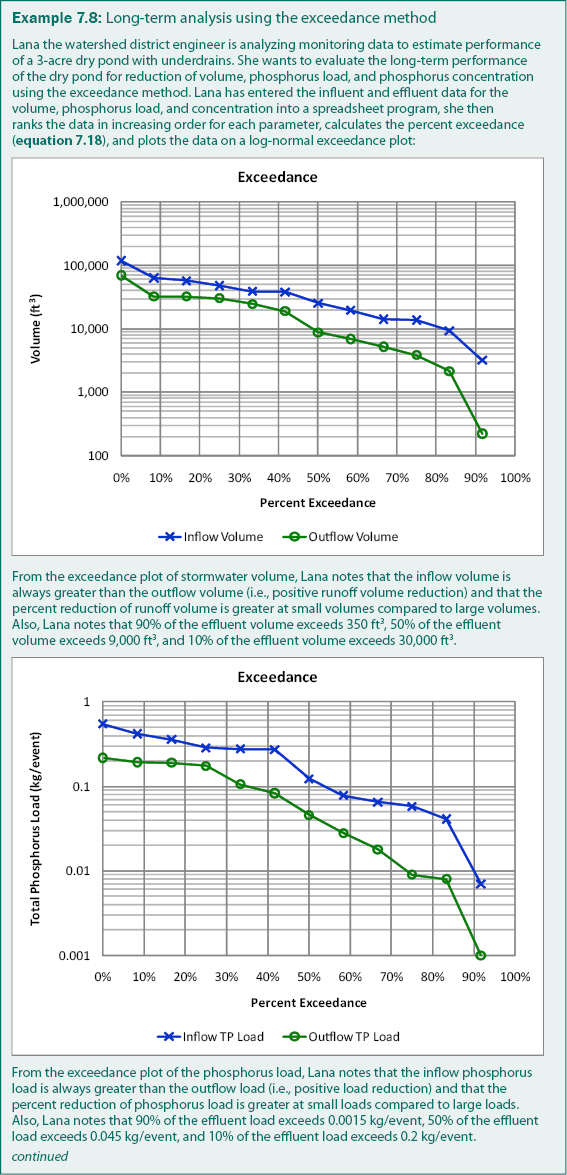
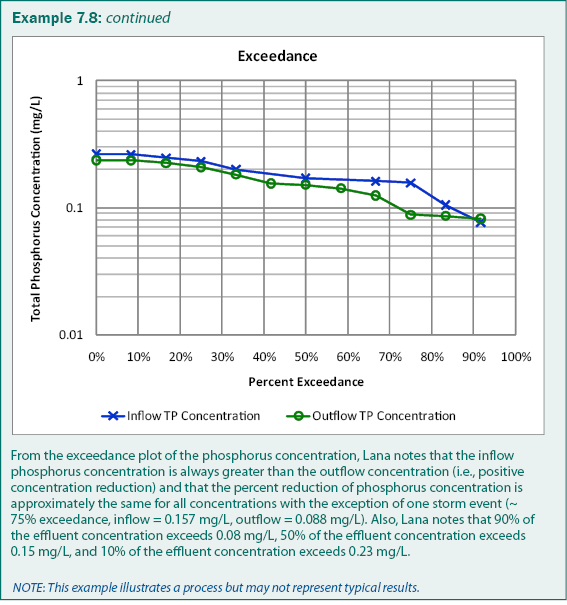
The exceedance method can be applied to any data including runoff volume, flow rate, pollutant concentration, pollutant load, residence time, and drain time. In addition to using storm event data such as event mean concentration and total pollutant load, individual sample and flow measurement data can be analyzed using the exceedance method. For example, all individual measurements of phosphorus concentration during individual storm events can be sorted, ranked, and plotted on an exceedance plot. Typically between five and fifty samples are collected during each storm event and when few storms have been assessed with monitoring, plotting all individual measurements on the exceedance plot can quickly illustrate trends in the data. The disadvantage is that the predictions or conclusions from this approach are limited to the range of storm events from which the data was collected and may not be appropriate for predicting performance for all possible storms, seasons, or conditions.

Effluent Probability Method

The U.S. EPA (2002) recommends using the effluent probability method for analysis of monitoring data. The effluent probability method is a graphical representation of long-term performance and is useful in visually illustrating trends in performance over the range of data values (e.g., runoff volume, flow rate, pollutant concentration, or pollutant load). The effluent probability method does not, however, result in a single value of performance for easy comparison to other monitoring data (other sites, time periods, etc.). Therefore, comparison of monitoring data using the effluent probability method is typically limited to graphical comparison (e.g., plotting inflow and outflow for multiple practices). Pollutant removal can be estimated by integrating the curve or best-fit distribution function for both the inflow and outflow data, and then calculating the difference between in the inflow and outflow. Due to the complexity of this method, it is more common to report performance for several probabilities (i.e., inflow and outflow data for 10%, 50%, and 90% probabilities).

One advantage of the effluent probability method is that monitoring data is plotted on a standard parallel probability plot which results in a straight line if the measurements are normally (normal-probability plot) or log-normally (log-probability plot) distributed. Also, the inflow and outflow data will be parallel if the percent difference between the inflow and outflow is constant for all ranked data pairs. One disadvantage, however, is that special software (e.g., MATLAB™) may be required to generate probability plots. In order to make defensible conclusions or predictions from the effluent probability method, several data points (at least 5; more than 10 recommended) are necessary. 

The primary difference between the effluent probability method and the exceedance method is that plotting the data using the exceedance method can be done using most commercially available spreadsheet software (e.g., Microsoft Excel™). One disadvantage of the exceedance method is that the normality of the data cannot be assessed visually.

Continue to Recommendations.